Detecting Placer Gold Mining from Sentinel-2 & Sentinel-1
A multi-method, multi-sensor change-detection pipeline for the Uylgaiin Dugang site, Mongolia.
Abstract
Placer gold mining in northern Mongolia leaves distinctive optical and radar signatures along river corridors: vegetation stripping, dredge ponds, exposed tailings, sediment plumes, and persistent loss of InSAR coherence. We combine freely-available Sentinel-2 multispectral and Sentinel-1 SAR imagery into a layered detection pipeline at the Uylgaiin Dugang site (49.78°N, 107.84°E). The pipeline starts from a multi-index Z-score change detector, layers in SAR coherence-loss fusion, applies AROSICS sub-pixel co-registration to remove geometric false positives along riverbanks, and culminates in a temporally dense time-series cube analysed by joint spectral-temporal PCA with a per-pixel change-point detector that identifies the moment a pixel switches from one terrain class to another. Cloud handling is unified across stages: SCL masking, dilated cloud edges, frame drop based on AOI valid fraction, and a temporal MAD outlier filter.
This document is interactive. Each method section has a "Theory of the method →" button that opens a deep-dive popup with the underlying math, algorithm pseudo-code, and a small SVG diagram. Click any of them whenever you want the derivation; ignore them and read the prose if you do not.
§ 1 The Site & the Problem
Placer gold mining strips a river corridor of vegetation, dredges the alluvium, dumps the rejected gravel as tailings, and leaves behind a chain of turbid settling ponds. From space, every one of those steps is visible — if you know which spectral indices to combine and how to filter out the natural seasonal cycle. Our test site is Uylgaiin Dugang in Töv Province, Mongolia (49.7767°N, 107.8357°E), an active placer site whose extent grew measurably between 2017 and 2020. The AOI is a tight 5×4.5 km box in EPSG:32648 (UTM zone 48N).
| Parameter | Value |
|---|---|
| Site name | Uylgaiin Dugang Mining |
| Centre (lat, lon) | 49.7767°N, 107.8357°E |
| AOI bbox (EPSG:4326) | [107.80, 49.76, 107.87, 49.80] |
| Reference grid | EPSG:32648 (UTM 48N), 10 m |
| Mining season | Apr–Dec, peak Jun–Aug |
| Baseline window | Jun–Aug 2017 |
| Peak-activity window | Jun–Aug 2020 |
Why off-the-shelf change detection is not enough
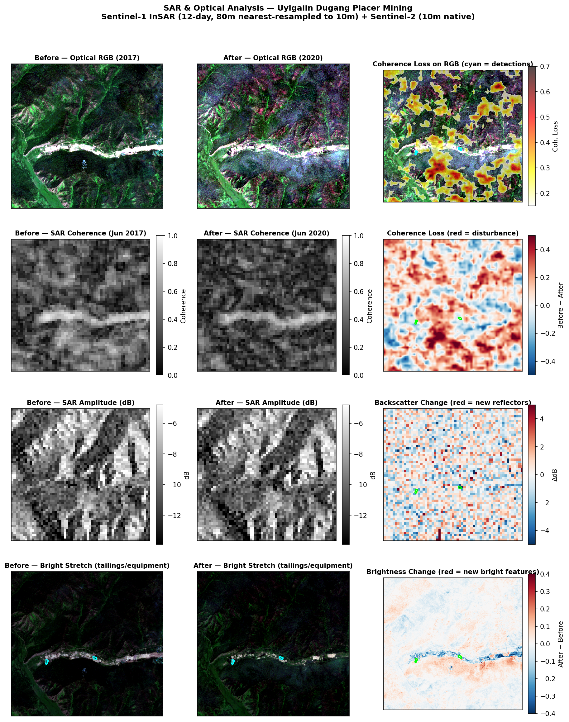
A naive Δ-NDVI between two summer composites flags everything: snow patches that haven't melted, cloud shadows the SCL classifier missed, fields harvested at different dates, and the natural sub-pixel drift of the Copernicus reference grid between processing baselines. Below the noise floor sits the actual mining signal, which has three properties that distinguish it: (a) it sits along a river corridor, (b) it persists rather than recovering, and (c) the optical signature is corroborated by SAR coherence loss because the dredge head physically moves. The pipeline below is built around these three properties.
§ 2 Data Sources
All sensors used are free at the point of access. The pipeline scaffolds a fifth (PlanetScope 3 m via the Planet Education & Research program) for the user's pending application, but every figure in this document is generated from the four free sources alone.
| Sensor | Bands / Mode | Resolution | Revisit | Role in pipeline |
|---|---|---|---|---|
| Sentinel-2 L2A | 13 bands incl. SWIR (B11, B12) | 10–20 m | ~5 d | Optical backbone — spectral indices, time-series cube |
| Sentinel-1 SLC | C-band IW, VV+VH, complex | ~5×20 m | ~12 d | InSAR coherence loss via ASF HyP3 |
| Sentinel-1 GRD | C-band IW backscatter | 20 m | ~12 d | dB-change for "new bright reflectors" (equipment, structures) |
| ALOS PALSAR mosaic | L-band HH/HV annual | 25 m | annual | Long-term mining-area expansion trend |
| PlanetScope SuperDove (scaffolded) | 8 bands, no SWIR | 3 m | ~daily | Pending Planet E&R access — sub-pit detail |
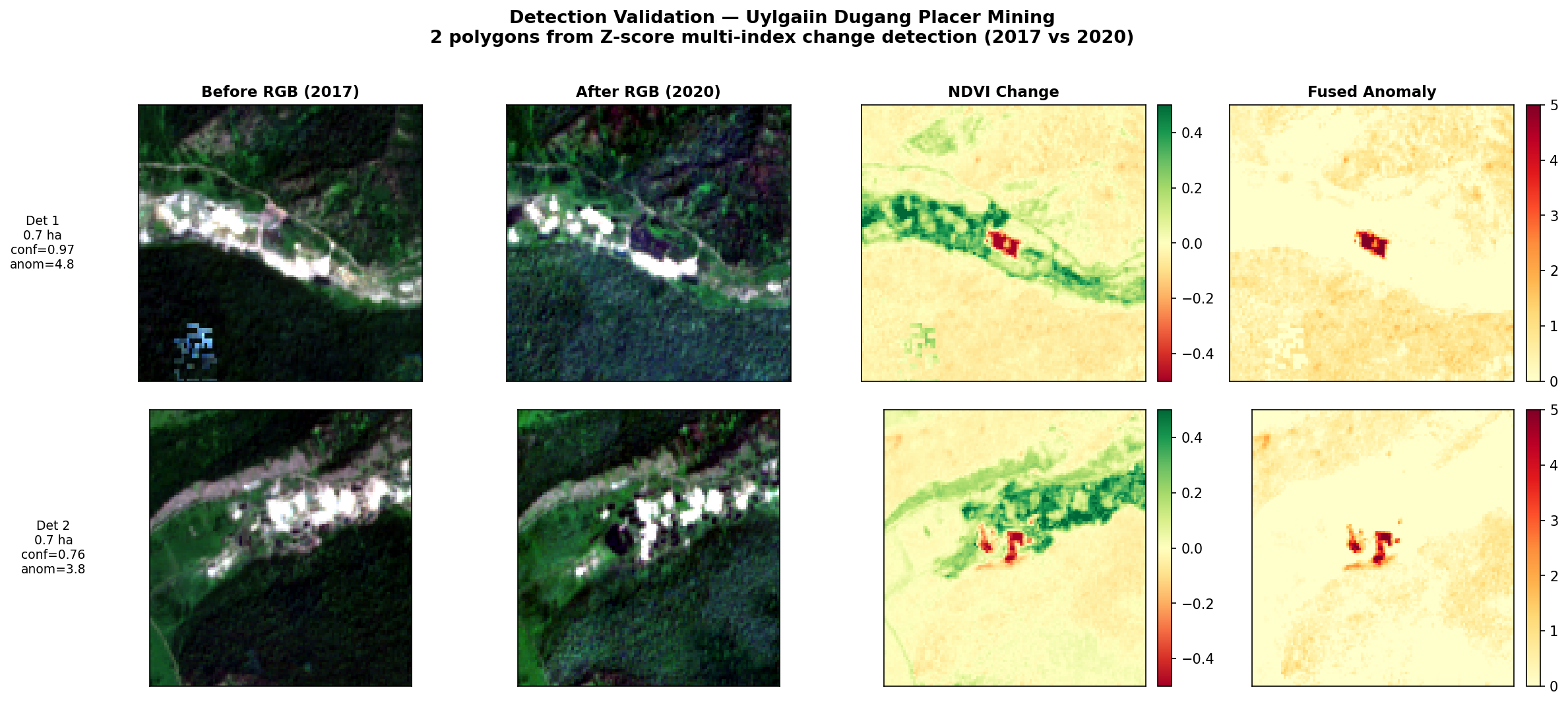
§ 3 Multi-Index Z-Score Change Detection
The first detector layer compares two Sentinel-2 median composites (Before, After), computes six spectral indices for each, takes the differences, standardizes per index, and weighted-sums them into a single anomaly map. The map is thresholded, morphologically cleaned, vectorised into polygons, and given a confidence boost if the polygon sits near a pre-existing water feature (placer mining hugs rivers).
| Index | Formula | Mining signature | Sign in fusion |
|---|---|---|---|
| NDVI | (NIR − R) / (NIR + R) | Vegetation stripping → large negative Δ | inverted |
| MNDWI | (G − SWIR1) / (G + SWIR1) | New ponds, dredge water → large positive Δ | positive |
| BSI | ((SWIR1+R) − (NIR+B)) / (sum) | Bare soil / tailings → positive Δ | positive |
| NDTI | (R − G) / (R + G) | Sediment plumes / turbidity → positive Δ | positive |
| NDWI | (G − NIR) / (G + NIR) | Open water increase → positive Δ | positive |
| NBR | (NIR − SWIR2) / (NIR + SWIR2) | General disturbance / burn → negative Δ | inverted |
§ 4 Optical × SAR Fusion
The optical Z-score detector struggles in two situations: (a) summer cloud cover blanks out critical Jun–Aug acquisitions, and (b) early-season false positives along snowmelt edges. Sentinel-1 InSAR coherence is independent of clouds and cleanly highlights "actively-disturbed ground": stable steppe maintains coherence >0.7 between repeat passes; an active dredge drops below 0.3. We fuse the two by adding a SAR boost on top of the optical Z-score.
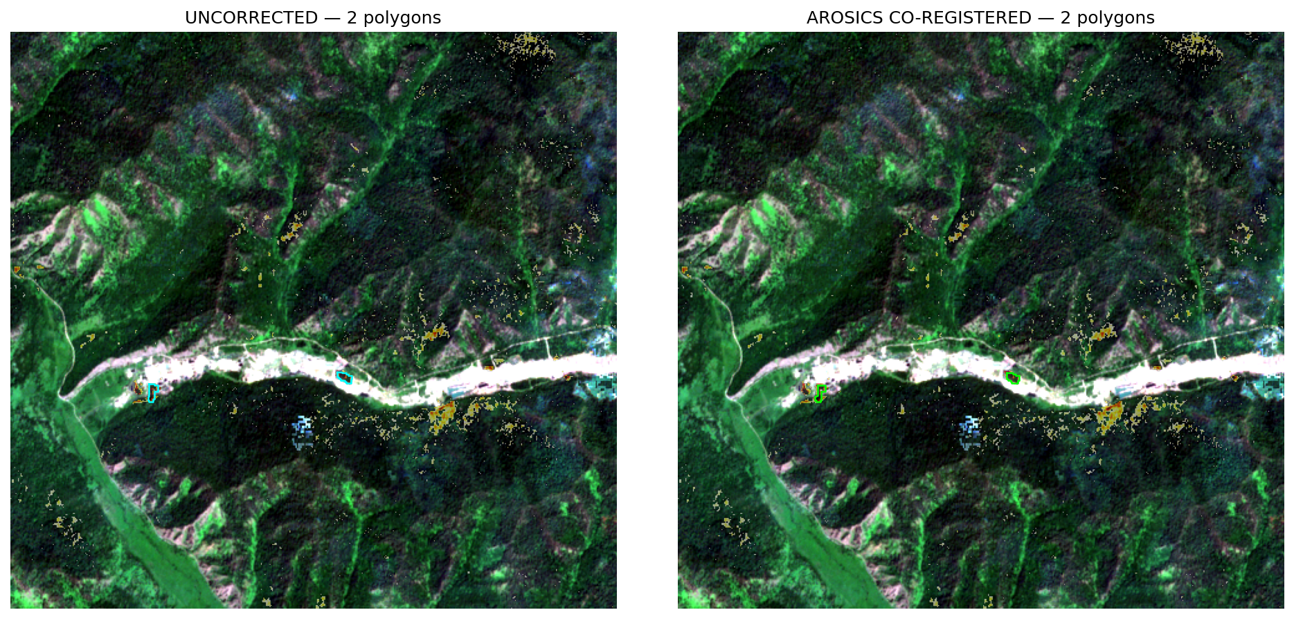
§ 5 Sub-Pixel Co-Registration
Sentinel-2 L2A products inherit Copernicus's global reference grid, but residual sub-pixel drift of even ~3 m produces visible "edge halos" along narrow rivers in the ΔMNDWI map and is the dominant source of false positives in riverine change detection. We benchmark seven co-registration methods in a separate CoRegistration project and pick AROSICS Global as the production aligner: it estimates a single rigid (Δx, Δy) translation in image-space using FFT phase correlation on a stable matching band (NIR), so it removes geometric mis-registration without absorbing real channel motion into a deformation field.
§ 6 Temporal PCA & Change-Point Detection
The before/after pipeline above only sees two snapshots per year. To exploit the full Sentinel-2 cadence we build a temporally dense data cube: every available S2 L2A scene over a one-year window, SCL-masked, AROSICS-aligned to a single reference, cloud-cleaned (dilation + frame drop + temporal MAD outlier rejection), and resampled onto a regular 5-day temporal grid. The result is a 4-D array $X \in \mathbb{R}^{T \times B \times H \times W}$ with $T \approx 36$ timesteps, $B = 6$ spectral bands, and ~243k pixels.
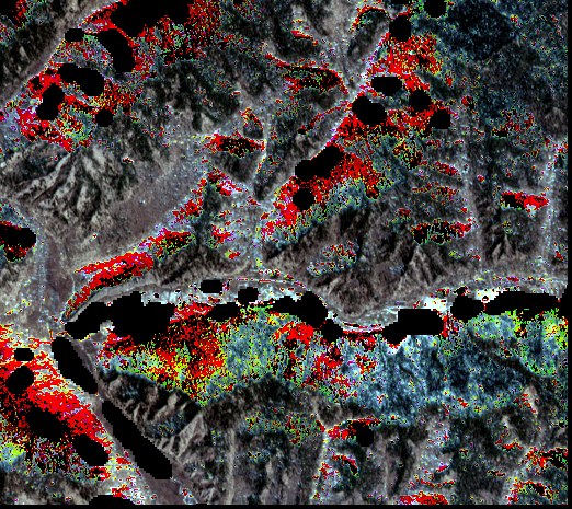
We then run joint spectral-temporal PCA: per pixel, stack all bands and times into a length-$TB$ "spectral-temporal fingerprint", standardize, build the $TB \times TB$ covariance, and eigendecompose. The principal components are length-$TB$ patterns that capture the dominant modes of how a pixel evolves over the year. Pixels sharing the same dominant PC share a temporal land-cover class — water, vegetation, snow, bare soil, mining. A per-pixel sliding-window detector then finds the time at which the dominant PC switches, which is exactly the question "when did this pixel stop behaving like X and start behaving like Y?"
§ 7 Results & Validation Numbers
Headline numbers (test_2020 cube, 6-month window)
- Raw STAC search: 49 S2 L2A items → 39 unique-date scenes after dedup
- Cloud cleanup: 17 of 39 scenes pass after dilation + 85% AOI valid threshold
- Cube shape: $T = 36 \times B = 6 \times 465 \times 522$ pixels on the 10 m UTM grid
- Cube NaN fraction: 28.86% raw → 2.21% interpolated
- Joint PCA explained variance: PC1 = 73.4%, top-5 cumulative = 86.4%
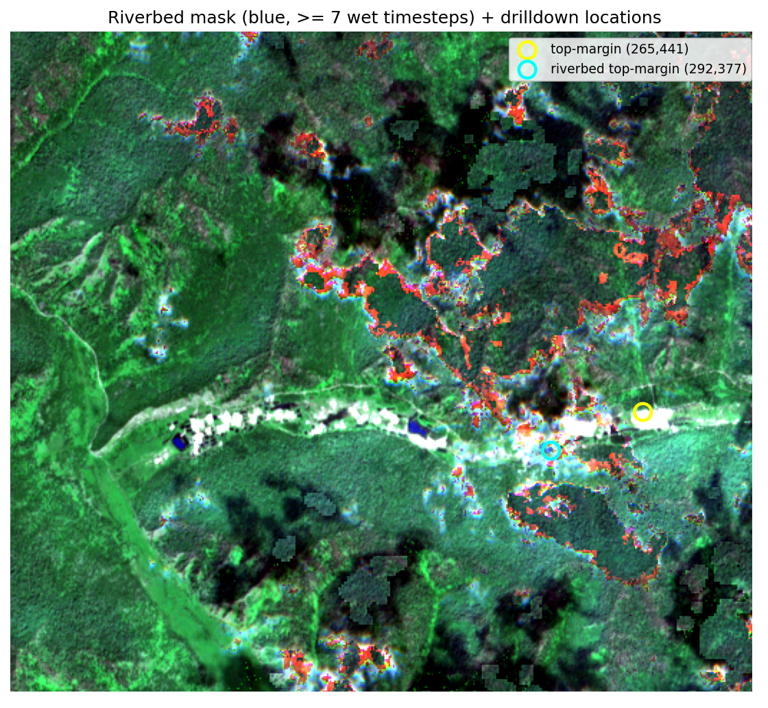
- Change events at margin ≥ 0.20: 3,057 pixels (1.26% of AOI)
- Top-margin change pixel: $(265, 441)$, 2020-04-22, PC3 → PC1, margin 0.397
- Riverbed top-margin pixel: $(292, 377)$, 2020-05-07, PC2 → PC1, margin 0.260
detections.geojson.
Where the cloud filter mattered most
Before adding the cloud-cleanup stage to timeseries_cube.py, the joint PCA was
dominated by cirrus and cloud-edge artefacts: PC1 captured only 30% of the variance and
the change-point detector flagged 35% of the AOI. The drilldown popups looked like clouds.
After dilating the SCL mask by 2 px, dropping any frame with <85% valid AOI pixels,
and rejecting per-pixel temporal outliers above 4·MAD, PC1 jumped to 73% of variance,
the change-pixel count fell to 1.26% of the AOI, and the surviving drilldowns are real
ground transitions instead of cloud edges. The per-frame KEEP/DROP decisions are logged
to cube_meta.json for audit.
§ 8 Next Steps
- Run on the full year. The pipeline scales linearly: 70–75 unique-date Sentinel-2 scenes over a 1-year window are downloaded, AROSICS-aligned, cloud-cleaned, and fed into the temporal-PCA cube without any code changes — just a bigger label.
-
PlanetScope SuperDove (3 m, daily) via the Planet Education &
Research program. The downloader and PlanetScope-specific change detector are already
scaffolded under
download_planetscope.pyandchange_detection_planetscope.py; they wait on API key issuance. With 3 m daily we move from "blob detection" to per-dredge tracking. - Refine the AROSICS local mode in the companion CoRegistration project. The temporal-PCA cube is currently aligned via AROSICS Global (a single rigid translation); swapping in the locally-varying Bayesian-tiled aligner would handle pairs across very different baseline reprocessings.
- Label the joint PCs by hand. The change-point detector reports "PC1 → PC7" transitions; an interpretive table mapping each PC to a temporal class ("snow-melt", "stable steppe", "disturbed bare ground" ...) would allow filtering for the specific transitions diagnostic of mining onset.